Implementing our Bayesian NFL Win Probability Model in Python

Predicting NFL Win Probabilities with PyMC: A Bayesian Hierarchical Approach

By Matt Rosinski

In our previous article, we explored how to predict NFL win probabilities using a Bayesian hierarchical model built with Stan. We incorporated crucial factors like score differential, time remaining, field position, and team effects to enhance our predictions. In this installment, we'll take a step further by implementing the same model using PyMC, a powerful Python library for Bayesian statistical modeling.

Our focus will be on:

1. Comparing the structure of the model in PyMC and Stan: Highlighting the similarities and differences.

2. Discussing the pros and cons of scaling continuous variables: Understanding its impact on Bayesian models.

3. Leveraging model visualization tools with ArviZ: Enhancing our interpretation of the model.

4. Comparing win probability predictions: Demonstrating the consistency of results across platforms.

---

Why Transition to PyMC?

While Stan is a robust platform for Bayesian modeling, Python's PyMC offers several advantages:

• Flexibility and Accessibility: Python's widespread use makes PyMC accessible to a larger audience.

• Integration with Python Ecosystem: Seamless integration with libraries like NumPy, pandas, and SciPy.

• Advanced Sampling Algorithms: PyMC utilizes state-of-the-art algorithms like the No-U-Turn Sampler (NUTS).

• Visualization with ArviZ: Powerful tools for diagnostics and result visualization.

---

Data Preparation

Before diving into the modeling, we need to prepare our data. We'll use the same dataset from our previous article, which includes play-by-play data from the 2023 NFL season.

Note: For detailed data preparation steps, please refer to our previous article.

---

Building the Hierarchical Bayesian Model with PyMC

1. Importing Libraries

import pandas as pd
import numpy as np
import pymc as pm
import arviz as az
import matplotlib.pyplot as plt
import seaborn as sns
from scipy.special import expit  # For the inverse logit function
from sklearn.preprocessing import StandardScaler

2. Loading and Exploring the Data

data = pd.read_csv("pbp_outcomes_2023.csv")

# Quick data inspection
print(data.head())
print(data.info())
print(data.describe())

3. Preparing the Data

• Assigning Team Indices: We map each team to a unique index for modeling purposes.

teams = data['posteam'].unique()
teams_sorted = np.sort(teams)
team_to_index = {team: idx for idx, team in enumerate(teams_sorted)}
data['team_index'] = data['posteam'].map(team_to_index)

# Number of teams
K = len(teams_sorted)
print(f"Number of teams: {K}")

• Scaling Continuous Variables: We standardize the predictors to have mean zero and unit variance.

scaler = StandardScaler()
scale_cols = ['score_differential', 'minutes_remaining', 'yardline_100']
data[scale_cols] = scaler.fit_transform(data[scale_cols])

print(data[scale_cols].head())

4. Defining Predictors and Outcome

y = data['win_loss'].values
score_diff = data['score_differential'].values
time_remain = data['minutes_remaining'].values
field_pos = data['yardline_100'].values
team = data['team_index'].values

# Number of observations
N = len(data)
print(f"N (number of observations): {N}")

---

Modeling with PyMC

Similarities and Differences with Stan

Similarities:

• Model Structure: Both PyMC and Stan allow us to define probabilistic models using a similar syntax for priors, likelihoods, and hierarchical structures.

• Non-Centered Parameterization: We use non-centered parameterization for team effects in both models to improve sampling efficiency.

• Hierarchical Modeling: Both platforms support hierarchical models, enabling partial pooling.

Differences:

• Syntax and Language: Stan uses its own modeling language, while PyMC models are built using Python code.

• Sampling Algorithms: While both use Hamiltonian Monte Carlo (HMC) methods, the implementation details differ.

• Model Compilation: Stan models require compilation, whereas PyMC models are interpreted directly in Python.

1. Defining the Model in PyMC

with pm.Model() as model:
    # Priors
    alpha = pm.Normal('alpha', mu=0, sigma=5)
    beta_score = pm.Normal('beta_score', mu=0, sigma=2)
    beta_time = pm.Normal('beta_time', mu=0, sigma=2)
    beta_field = pm.Normal('beta_field', mu=0, sigma=2)
    
    mu_team = pm.Normal('mu_team', mu=0, sigma=1)
    sigma_team = pm.HalfNormal('sigma_team', sigma=1)
    
    # Team effects (non-centered parameterization)
    team_effect_raw = pm.Normal('team_effect_raw', mu=0, sigma=1, 
                                 shape=K)
    team_effect = pm.Deterministic('team_effect', mu_team + sigma_team * 
                                    team_effect_raw)
    
    # Linear predictor
    eta = (alpha +
           beta_score * score_diff +
           beta_time * time_remain +
           beta_field * field_pos +
           team_effect[team])
    
    # Likelihood
    y_obs = pm.Bernoulli('y_obs', logit_p=eta, observed=y)

2. Sampling from the Posterior

with model:
    idata = pm.sample(
        tune=2000,
        draws=2000,
        cores=4,
        chains=4,
        target_accept=0.95,
        return_inferencedata=True
    )

---

Scaling Continuous Variables: Pros and Cons

Pros of Scaling

• Numerical Stability: Scaling helps in achieving numerical stability during sampling, especially when predictors are on different scales.

• Improved Convergence: Scaled variables often lead to faster convergence and more efficient sampling.

• Interpretability of Priors: When variables are standardized, priors on coefficients can be more meaningfully specified.

Cons of Scaling

• Interpretation Difficulty: Coefficients of scaled variables represent the effect per standard deviation, which may be less intuitive.

• Additional Complexity: Requires keeping track of scaling parameters to transform new data or interpret results.

Conclusion: In Bayesian modeling, especially with HMC methods, scaling is generally beneficial and recommended for continuous predictors.

---

Model Visualization with ArviZ

ArviZ is a Python package for exploratory analysis of Bayesian models, offering diagnostic plots and statistical summaries.

1. Model Graph

pm.model_to_graphviz(model)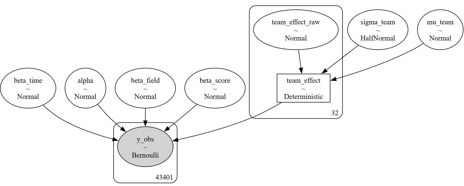

Model graph

2. Trace Plots

az.plot_trace(idata, var_names=['alpha', 'beta_score', 'beta_time', 'beta_field', 'mu_team', 'sigma_team'])
plt.show()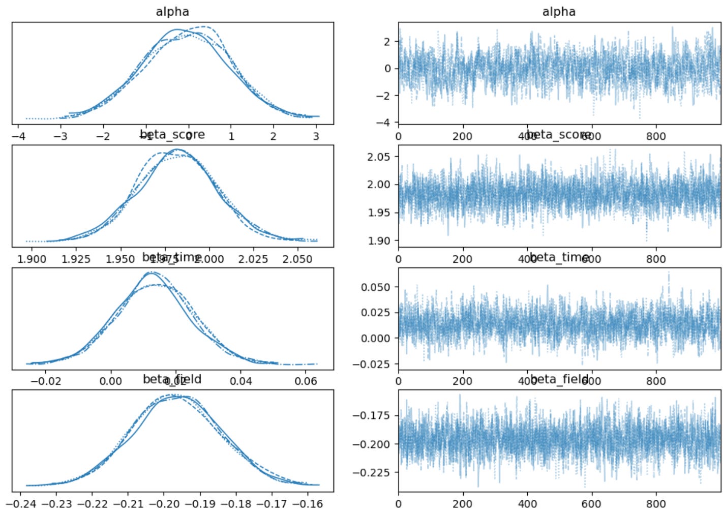

Model parameter trace plots

Trace plots help assess convergence and mixing of the chains.

---

Predicting Win Probabilities

1. Defining the Scenario

For a direct comparison with the model we built using Stan, let's predict the win probabilities for a scenario where a team is down by 6 points with 10 minutes remaining at their own 30-yard line.

# Original (unscaled) scenario parameters
score_diff_unscaled = -6
time_remain_unscaled = 10
field_pos_unscaled = 70  # Yardline is measured as yards from the opponent's end zone

# Scaling the scenario using the same scaler
scenario_scaled = scaler.transform([[score_diff_unscaled, time_remain_unscaled, field_pos_unscaled]])
score_diff_scaled = scenario_scaled[0, 0]
time_remain_scaled = scenario_scaled[0, 1]
field_pos_scaled = scenario_scaled[0, 2]

print(f"Scaled Scenario Parameters:\nScore Differential: {score_diff_scaled}\nTime Remaining: {time_remain_scaled}\nField Position: {field_pos_scaled}")

2. Computing Win Probabilities

# Extract posterior samples
posterior = idata.posterior
alpha_samples = posterior['alpha'].values.flatten()
beta_score_samples = posterior['beta_score'].values.flatten()
beta_time_samples = posterior['beta_time'].values.flatten()
beta_field_samples = posterior['beta_field'].values.flatten()
team_effect_samples = posterior['team_effect'].values  # Shape: (chains, draws, K)
team_effect_samples = team_effect_samples.stack(draws=("chain", 
                                                       "draw")).values

# Compute win probabilities for each team
win_probs = pd.DataFrame()
for team_idx, team_name in enumerate(teams_sorted):
    team_effect = team_effect_samples[:, team_idx]
    log_odds = (alpha_samples +
                beta_score_samples * score_diff_scaled +
                beta_time_samples * time_remain_scaled +
                beta_field_samples * field_pos_scaled +
                team_effect)
    win_prob = expit(log_odds)
    win_probs[team_name] = win_prob

---

Visualizing Win Probabilities

Win Probability Distribution by Team

We visualize the distribution of win probabilities for each team.

# Order teams by mean win probability
mean_win_probs = win_probs.mean().sort_values(ascending=False)
ordered_teams = mean_win_probs.index.tolist()

# Melt the DataFrame for plotting
win_probs_melted = win_probs.melt(var_name='Team', value_name='Win_Probability')
win_probs_melted['Team'] = pd.Categorical(win_probs_melted['Team'], categories=ordered_teams, ordered=True)

# Plotting
plt.figure(figsize=(10, 12))
sns.violinplot(
    data=win_probs_melted,
    y='Team',
    x='Win_Probability',
    order=ordered_teams,
    inner='quartile',
    palette='muted'
)
plt.title('Win Probability Distribution by Team\nScenario: Down by 6 Points with 10 Minutes Remaining at Own 30-yard Line', fontsize=16, pad=20)
plt.xlabel('Win Probability', fontsize=14)
plt.ylabel('Team', fontsize=14)
plt.tight_layout()
plt.show()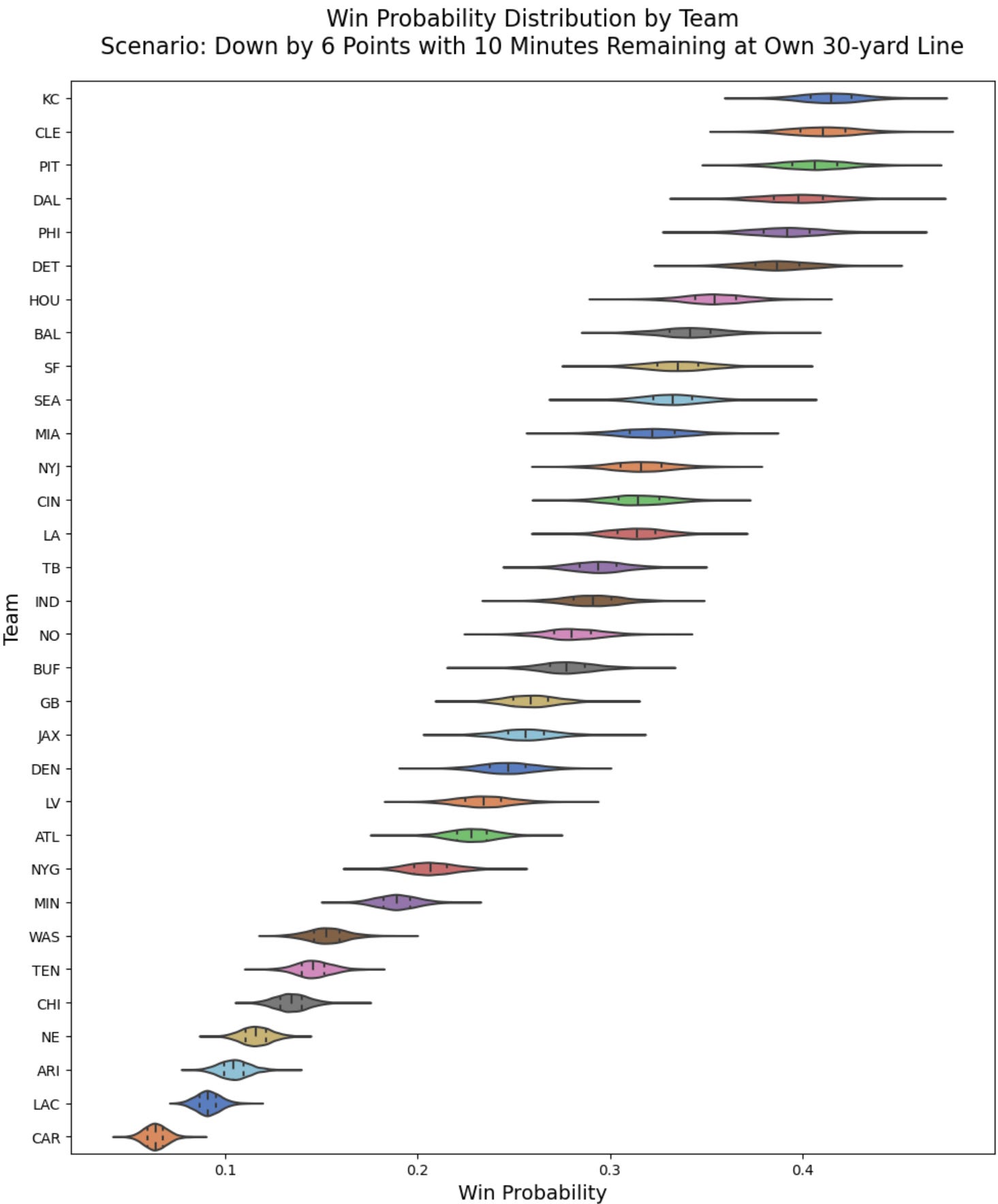

Win Probability for Scenario with Team Effects

• Team Strength: Teams with higher average win probabilities may be considered stronger in such situations.

• Uncertainty: The width of the distributions reflects the uncertainty in the predictions.

---

Comparing Results with the Stan Model

Despite using different platforms, the PyMC and Stan models produce similar win probability distributions. Compare the plot above with the comparable distributions from the previous model built using Stan. This consistency reinforces the robustness of our Bayesian hierarchical approach.

Key Takeaways:

• Model Structure: Both models leverage partial pooling and non-centered parameterization.

• Scaling: Standardizing variables aids in model convergence and comparability.

• Visualization: Tools like ArviZ and Seaborn facilitate insightful analysis of model outputs.

---

Conclusion

Transitioning our Bayesian hierarchical model from Stan to PyMC has allowed us to harness Python's rich ecosystem while maintaining the integrity of our predictions. By carefully scaling our variables and utilizing ArviZ we can easily visualize the model graph, trace plots and more.

---

Interested in a Masterclass in building Bayesian models with sports data? Check out Dr. Scott Spencer's fantastic Becoming a Bayezian course. I highly recommend it.