Expanding on our Bayesian NFL Win Probability Model

How to build a hierarchical Bayesian model (and include team-specific effects on win probability)

By Matt Rosinski

---

Predicting the outcome of an NFL game at any given moment is a complex task that involves understanding various dynamic factors such as the score differential, time remaining, field position, and team strengths. In this article, we'll extend the Bayesian model we built in the previous issue to estimate a more representative win probability for a team given these factors. Again we'll leverage play-by-play data from the 2023 NFL season and utilize modern Bayesian techniques to capture uncertainty and provide insightful predictions.

Introduction

Traditional statistical models often struggle to account for the inherent uncertainties and variations in sports data. Bayesian models, on the other hand, allow us to incorporate prior knowledge and quantify uncertainty in our predictions. By using a hierarchical Bayesian approach, we can model team-specific effects and understand how different factors contribute to the win probability.

In this article, we'll:

• Load and preprocess NFL play-by-play data.

• Build a hierarchical Bayesian model using Stan.

• Fit the model using the cmdstanr package in R.

• Visualize the posterior distributions of win probabilities for each team.

• Interpret the results and discuss potential applications.

---

Data Preparation

Loading Necessary Libraries

We'll start by loading the required R packages:

library(nflfastR)
library(tidyverse)
library(cmdstanr)
library(ggdist)
library(bayesplot)
library(posterior)
library(tidybayes)

For faster model fitting you can run on multiple cores:

# Assuming you have 8 cores available 
options(mc.cores = 8)

Loading the Play-by-Play Data

We use the nflfastR package to load the 2023 NFL play-by-play data. To optimize performance, we save the data locally using the arrow package:

# Load the play-by-play data for the 2023 season
pbp_2023_data <- load_pbp(2023)

Data Exploration

Let's take a quick look at the data structure:

glimpse(pbp_2023_data)

Filtering Relevant Plays

We focus on plays that can significantly impact the game's outcome:

pbp_filtered <- pbp_2023_data %>% 
  select(play_id, game_id, home_team, home_score, away_team, away_score,
         score_differential, game_seconds_remaining, yardline_100, 
         result, posteam, defteam, play_type, series_result) %>% 
  group_by(game_id) %>% 
  filter(play_type %in% c("pass","run","field_goal","punt","kickoff") | 
         score_differential != lag(score_differential, default = 0)) %>% 
  ungroup()

We then remove plays with missing essential data:

pbp_cleaned <- pbp_filtered %>% 
  drop_na(score_differential, game_seconds_remaining, yardline_100)

Feature Engineering

We need to create a binary outcome variable indicating whether the team in possession won the game. We'll determine the winning team based on the final score:

# Get the final scores for each game
game_outcomes <- pbp_cleaned %>%
  group_by(game_id) %>%
  filter(play_id == max(play_id)) %>%  # Get the last play in the game
  summarize(
    home_team = unique(home_team),
    away_team = unique(away_team),
    home_score = max(home_score),
    away_score = max(away_score)
  ) %>%
  mutate(
    winning_team = case_when(
      home_score > away_score ~ home_team,
      home_score < away_score ~ away_team,
      TRUE ~ NA_character_  # In case of a tie
    )
  ) %>%
  select(game_id, winning_team) %>%
  ungroup()

We merge this information back into our play-by-play data:

pbp_with_outcome <- pbp_cleaned %>% 
  left_join(game_outcomes, by = "game_id") %>% 
  mutate(
    win_loss = ifelse(posteam == winning_team, 1,
                      ifelse(is.na(winning_team), NA, 0)),
    minutes_remaining = game_seconds_remaining / 60
  ) %>% 
  filter(!is.na(win_loss))

---

Building the Bayesian Model

Understanding Hierarchical Models and Pooling

Before building the model, it's important to understand the concept of hierarchical models and the idea of pooling:

• Hierarchical Models: These models introduce group-level parameters to account for the hierarchical structure in the data. In our case, teams represent groups, and we expect that each team might have its unique characteristics affecting the win probability.

• Pooling:

  • Complete Pooling: Assumes all groups are the same; data from all groups are combined to estimate a single effect.

  • No Pooling (Unpooled): Estimates separate effects for each group without sharing information between them.

  • Partial Pooling: Shares information across groups while allowing for group-specific deviations. This is achieved through hierarchical modeling.

Our model uses partial pooling. By including team-specific effects with a common prior distribution, we allow each team's effect to be informed by both its own data and the overall league data. This approach balances between overfitting (no pooling) and underfitting (complete pooling), providing more reliable estimates, especially for teams with less data.

Setting Up the Data for Stan

We create an index for teams and prepare the data in the format required by Stan:

# Create team index
team_levels <- pbp_with_outcome$posteam %>% unique() %>% 
               sort()

model_data <- pbp_with_outcome %>%
  mutate(team_index = as.integer(factor(posteam, levels = team_levels))) 
  %>% 
  mutate(
    score_diff_std = scale(score_differential),
    time_remain_std = scale(minutes_remaining),
    field_pos_std = scale(yardline_100)
  )

# Prepare Stan data list
dat <- list(
  N = nrow(model_data),
  y = model_data$win_loss,
  score_diff = model_data$score_differential,
  time_remain = model_data$minutes_remaining,
  field_pos = model_data$yardline_100,
  team = model_data$team_index,
  K = length(team_levels)
)

The Stan Model

We define a hierarchical logistic regression model with team-specific effects:

// Filename: pbp_win_prob_2.stan
data {
  int<lower=0> N;                       // Number of observations
  int<lower=1> K;                       // Number of teams
  array[N] int<lower=0, upper=1> y;     // Win outcome
  vector[N] score_diff;                 // Score differential
  vector[N] time_remain;                // Minutes remaining
  vector[N] field_pos;                  // Field position (yardline_100)
  array[N] int<lower=1, upper=K> team;  // Team indices
}
parameters {
  real alpha;                 // Intercept
  real beta_score;            // Coefficient for score differential
  real beta_time;             // Coefficient for time remaining
  real beta_field;            // Coefficient for field position
  real mu_team;               // Population mean of team effects
  real<lower=0> sigma_team;   // Standard deviation of team effects
  vector[K] team_effect_raw;  // Unscaled team effects
}
transformed parameters {
  vector[K] team_effect = mu_team + sigma_team * team_effect_raw;
}
model {
  // Priors
  alpha ~ normal(0, 5);
  beta_score ~ normal(0, 2);
  beta_time ~ normal(0, 2);
  beta_field ~ normal(0, 2);
  mu_team ~ normal(0, 1);
  sigma_team ~ normal(0, 1);
  team_effect_raw ~ normal(0, 1);

  // Linear predictor
  vector[N] eta;
  eta = alpha + beta_score * score_diff +
        beta_time * time_remain + beta_field * field_pos +
        team_effect[team];

  // Likelihood
  y ~ bernoulli_logit(eta);
}

Compiling and Fitting the Model

We compile the Stan model and fit it using cmdstanr:

# Compile the model
m_pbp2 <- cmdstan_model("pbp_win_prob_2.stan")

# Fit the model
f_pbp2 <- m_pbp2$sample(data = dat)

Model Diagnostics

We now check the convergence diagnostics and visualize the parameter traces:

# Summarize the fit
summary_fit <- f_pbp2$summary()

# Generate trace plots for visual inspection
mcmc_trace(f_pbp2$draws(), 
           pars = c("alpha","beta_score", "beta_time", "beta_field"))

# Check for convergence issues
f_pbp2$cmdstan_diagnose()

---

Analyzing the Results

Extracting Posterior Samples

We can extract the posterior distributions of the model parameters as random variables (rvars):

# Extract posterior samples as rvars
posterior <- f_pbp2$draws(variables = c("alpha","beta_score", 
                          "beta_time", "beta_field","team_effect")) %>%
  as_draws_rvars()

Defining the Game Scenario

We set up a hypothetical game scenario to predict win probabilities:

• Score Differential: Down by 6 points

• Time Remaining: 10 minutes

• Field Position: At own 30-yard line (70 yards to the end zone)

# Scenario parameters
score_diff <- -6          # Down by 6 points
time_remain <- 10         # 10 minutes remaining
field_pos <- 70           # At own 30-yard line

Computing Win Probabilities

We then calculate the posterior win probability distributions for each team:

# Define inverse logit function compatible with rvars
inv_logit <- function(x) {
  1 / (1 + exp(-x))
}

team_df <- tibble(
  team = team_levels,
  team_index = 1:length(team_levels)
) %>%
  mutate(
    # Compute log-odds as an rvar for each team
    log_odds = posterior$alpha +
      posterior$beta_score * score_diff +
      posterior$beta_time * time_remain +
      posterior$beta_field * field_pos +
      posterior$team_effect[team_index],
    # Convert log-odds to win probability using inv_logit()
    win_prob = inv_logit(log_odds)
  )

---

Visualizing the Win Probabilities

We can use the ggdist and ggplot2 packages to visualize the posterior distributions of win probabilities for each team:

ggplot(team_df, aes(xdist = win_prob, y = reorder(team, mean(win_prob)))) +
  stat_halfeye(
    .width = c(0.5, 0.8, 0.95),
    slab_color = "steelblue",
    interval_color = "black",
    slab_alpha = 0.7
  ) +
  labs(
    title = "Win Probability Distribution by Team",
    x = "Win Probability",
    y = "Team",
    caption = "Scenario: Down by 6 points with 10 minutes remaining at 
               own 30-yard line"
  ) +
  theme_minimal()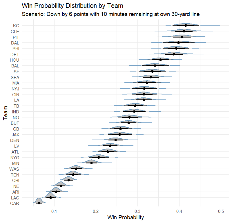

This plot shows:

• Density Plots: The distribution of win probabilities for each team.

• Credible Intervals: 50%, 80%, and 95% intervals indicating the uncertainty in the predictions.

• Team Ordering: Teams are ordered based on their mean win probability in this scenario.

---

Interpreting the Results

The Bayesian model provides probabilistic estimates of a team's chance to win given the game situation. The hierarchical structure allows us to capture team-specific strengths and weaknesses.

• Score Differential: As expected, being down by 6 points decreases the win probability.

• Time Remaining: With 10 minutes left, there's still significant time to influence the game outcome.

• Field Position: Starting at the own 30-yard line requires advancing the ball significantly to score.

Team Effects

The team-specific effects (team_effect) adjust the baseline probabilities based on each team's historical performance. Teams with stronger performances in similar situations such as Kansas City will have higher win probabilities.

---

Applications and Extensions

This model can be extended and applied in various ways:

• Real-Time Win Probability: Update predictions throughout a game to provide live win probabilities.

• Decision Making: Assist coaches in making strategic decisions based on the likelihood of winning.

• Betting Markets: Inform betting odds with probabilistic estimates that account for uncertainty.

• Player-Level Analysis: Incorporate player-specific data to refine predictions.

---

Summary

By leveraging Bayesian hierarchical modeling, we've developed a robust approach to predict NFL win probabilities that accounts for key game factors and team-specific effects. This method provides not only point estimates but also quantifies the uncertainty inherent in sports outcomes.

The flexibility of Bayesian models allows for continuous refinement and adaptation as more data becomes available. As we gather more seasons of data and include additional predictors, the model's accuracy and utility will continue to improve.

Ready to master Bayesian modeling? The Athlyticz comprehensive course on Bayesian Statistics will equip you with the skills to tackle real-world problems. Whether you're just starting out or aiming to refine your expertise, this course is designed for you. Enroll today and elevate your sports analytics game!