An Introduction to Bayesian Modeling for NFL Win Probabilities

How to estimate the chance your NFL team will win (even if they are ahead by 3 and there's only 10 minutes left In the game)

This article was written by Matt Rosinski. Matt is a Senior Data Scientist with a PhD in Engineering and has 25 years of experience working in academic research, industry and data science.

---

When watching an NFL game, one of the questions that might come up for you is, "What are the chances that my team will win given the current score and time left on the clock?" Intuitively, we understand that being ahead with little time remaining makes it more likely for a team to win. But how can we model this relationship mathematically?

In this article, I'll walk you through building a Bayesian model that estimates the win probability for an NFL team based on the score differential and the remaining time in the game. This tutorial assumes you have some familiarity with R and Bayesian modeling, but I'll guide you step by step through the process.

Step 1: Import Libraries and Load the Data

We start by importing necessary libraries and loading play-by-play (PBP) data from the 2023 NFL season.

library(nflfastR)
library(tidyverse)
library(cmdstanr)
library(ggdist)
library(bayesplot)
library(posterior)
library(tidybayes)

# Load play-by-play data for 2023 season
pbp_2023_data <- load_pbp(2023)

This play-by-play data contains detailed records of every event in a game, such as passes, runs, field goals, and more. It will provide us with the raw data we need to model win probability.

Step 2: Filter and Clean the Data

To build our model, we'll need to filter down the data to focus on key plays where the score changed, then clean it up for analysis.

pbp_filtered <- pbp_2023_data %>% 
  filter(play_type %in% c("pass", "run", "field_goal", "punt")) %>%
  select(play_id, game_id, home_team, away_team, score_differential, 
         game_seconds_remaining, posteam, defteam) %>% 
  group_by(game_id) %>%
  ungroup()

pbp_cleaned <- pbp_filtered %>% 
  drop_na(score_differential, game_seconds_remaining)

Here, we focus on key events like passes, runs, and field goals, which impact the score. We also filter out missing data to ensure we have a complete dataset for modeling.

Step 3: Feature Engineering

Next, we create a binary variable that represents whether the team in possession won or lost the game. This variable will be the target for our Bayesian model.

game_outcomes <- pbp_cleaned %>%
  group_by(game_id) %>%
  filter(play_id == max(play_id)) %>%  
  summarize(final_score_diff = max(score_differential), 
            posteam_final = posteam, 
            defteam_final = defteam) %>%
  mutate(winning_team = ifelse(final_score_diff > 0, 
                               posteam_final, 
                               defteam_final)) %>%
  ungroup()

pbp_with_outcome <- pbp_cleaned %>%
    left_join(game_outcomes, by = "game_id") %>%
    mutate(win_loss = ifelse(posteam == winning_team, 1, 0))

By adding this win_loss column, we now know the eventual winner for each game, which we can use to predict outcomes based on score differential and time remaining.

Step 4: Build the Bayesian Model

Now we're ready to specify our Bayesian model in Stan. The model assumes that the probability of winning depends on two main factors: the score differential and the time remaining.

dat <- list(
    N = nrow(pbp_with_outcome),
    score_differential = pbp_with_outcome$score_differential, 
    time_remaining = pbp_with_outcome$game_seconds_remaining,  
    win_loss = pbp_with_outcome$win_loss  
)

m <- cmdstan_model(stan_file = 'prob_win_differential.stan')

fit <- m$sample(
    data = dat,
    seed = 2024,
    chains = 4,
    iter_warmup = 1000,
    iter_sampling = 2000
)

In our Stan model, we specify priors that reflect our understanding of the problem. For instance, we assume that as the score differential increases, the likelihood of winning goes up, and as time remaining decreases, the likelihood of coming back diminishes.

Here's the full Stan code for the model:

data {
    int<lower=0> N;
    vector[N] score_differential;
    vector[N] time_remaining;
    array[N] int<lower=0, upper=1> win_loss;
}
parameters {
    real alpha;
    real beta_score;
    real beta_time;
}
model {
    alpha ~ normal(0, 2);
    beta_score ~ normal(0.1, 0.05);
    beta_time ~ normal(-0.001, 0.001);
    win_loss ~ bernoulli_logit(alpha + beta_score * score_differential + beta_time * time_remaining);
}

Step 5: Interpret Results

After fitting the model, we can extract posterior samples for our parameters (alpha, beta_score, and beta_time) and use them to predict win probability given different game scenarios.

posterior_samples <- fit$draws(c("alpha", "beta_score", "beta_time"))

posterior_samples_df <- posterior_samples %>%
    spread_draws(alpha, beta_score, beta_time)

predict_win_probability <- function(posterior_samples_df, 
                                    score_differential, 
                                    time_remaining){
  alpha <- posterior_samples_df$alpha
  beta_score <- posterior_samples_df$beta_score
  beta_time <- posterior_samples_df$beta_time
  
  logit_p <- alpha + beta_score * score_differential + beta_time * time_remaining
  p_win <- 1 / (1 + exp(-logit_p))
  
  return(p_win)
}

Step 6: Visualize Win Probability

Finally, we can visualize how win probability changes with score differential and time remaining.

plot_win_probability <- function(score_diff, seconds_remaining){
  
  tibble(win_prob = predict_win_probability(posterior_samples_df, 
                                            score_diff, 
                                            seconds_remaining)) %>% 
    ggplot(aes(x = win_prob)) +
    stat_dots(quantiles = 100) +
    labs(
      title="Win probability for NFL team in possession",
      subtitle=paste0("Leading by ", score_diff, " with ", 
                      round(seconds_remaining/60)," minutes remaining"),
      x = "Win Probability",
      y = "Frequency"
    ) +
    theme_bw()
}

plot_win_probability(3, 600)  # Leading by 3 with 10 minutes remaining
plot_win_probability(-3, 30)  # Trailing by 3 with 30 seconds remaining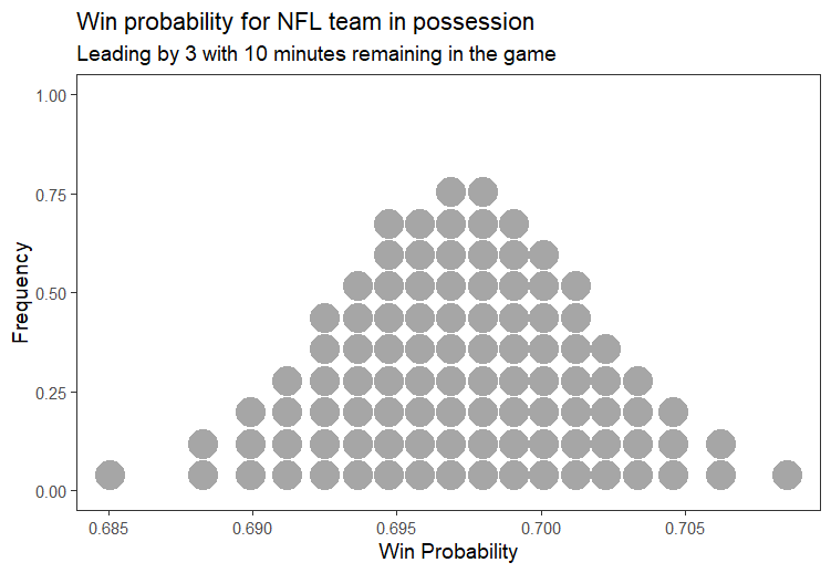

Fig 1: The model predicts there is a 69 to 70.5% chance of a team winning when leading by 3 with 10 min remaining.

The model predicts that there is around a 70% chance that a team leading by 3 points who is in possession with 10 minutes remaining will win the game. But of course there are many other factors that will influence their chances, such as where they are on the field and in the play sequence. We can certainly improve upon this model.

Fig 2: The model predicts there is between a 41 and 43.5% chance of a team winning trailing by 3 with 30 seconds remaining.

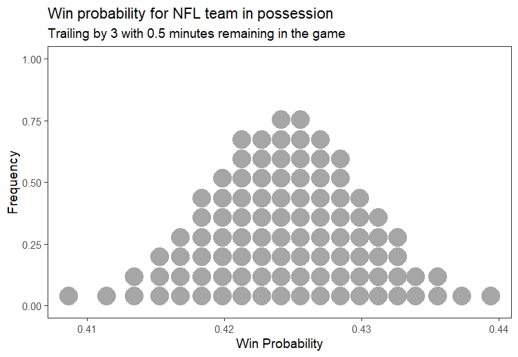
Likewise, you might think that the probability of winning when behind by 3 with 30 seconds shown in Figure 2 is a little too high. But what if the team is at the 10 yard line on the 2nd down with 30 seconds remaining on the clock? Now you might feel that the chances of winning if 3 points down with 30 seconds to go might be higher than 42.5%.

Ways we might improve our model might include adding more predictors like field position, strength of the defensive team and many other factors that may influence the chance of winning. Our goal here, is to give you a glimpse of what is possible.

Conclusion

This Bayesian approach offers a flexible and powerful way to model win probability in NFL games. The beauty of Bayesian modeling is that it provides full probability distributions for all parameters, which allows for uncertainty quantification — key in making informed decisions in sports or any other domain.

If you're excited by this example and want to dive deeper into Bayesian modeling, we offer a comprehensive course on Bayesian Statistics, where you'll learn how to apply these techniques to real-world problems yourself. Whether you're new to the field or looking to sharpen your skills, this course is perfect for you. Check us out at athlyticz.com and take your data science journey to the next level!